
What separates success from failure—in every business, in every marker—is timing. Every business owner, every operator, every financial manager knows WHAT to do. They just don’t know WHEN to do it. The cost of getting the timing wrong is catastrophic. A retailer who reorders late loses the sale. A restaurant that overpreps eats the margin. A manufacturer who ramps early bleeds cash. A fund manager who buys at the wrong time loses the fund. Solving the timing problem is the sole purpose of forecasting.
The source of the timing problem is that every application of time series forecasting generates a Prediction, not a Forecast.
A Prediction is a single-outcome call about the future.
It states what will happen as one definite outcome at a specific point in time, with no probability content attached. The Prediction is either right or wrong when the time arrives. A Prediction collapses the future into a single outcome with no surrounding context: no measure of how likely the outcome is, no range of what else could occur, no specification of what counts as normal at that position. Without that context, the Prediction cannot support a decision. The operator has no basis to hedge, to size inventory or capital against variation, or to allocate a risk budget, because none of those decisions can be made against a single number. A Prediction tells you WHAT the number will be. It cannot tell you WHEN that number is not normal and requires action, because it carries no definition of normal against which the value could be flagged.
Prediction intervals and confidence intervals are sometimes overlaid on Predictions to suggest probability content, but they do not deliver what they appear to claim. Both are computed from the predicting model’s own residuals and extrapolated forward; they describe how well the model fit its training data, not how often future outcomes will land within the band. Neither is verified against actual future outcomes, because the model that produced the Prediction is the same model whose fit determines the band’s width. The bands look like probability content, but operationally they are decoration on a single-outcome call.
A Forecast is a probability distribution over what can actually happen, attached to a specific point in time.
The probabilities of a Forecast are calibrated against actual outcomes observed over many independent cycles. The Forecast tells you not only what might happen but also how often each outcome actually happens at this point in the cycle, based on the historical track record of the forecasting process itself. The Calibrated Probability Band (CPB) is verified probability content: across the historical record, the 85% band has contained 85% of observations, the 90% band has contained 90%, and so on. The label states what the band delivers; the historical record confirms it. A Forecast engages with three orthogonal dimensions: Timeline (dim 6) as the structural temporal dimension, Probability (dim 5) as the dimension where multiple possible viewpoints (perspectives) coexist as superpositions, and Perspective (dim 4), the resolved value or outcome. A Forecast object includes the complete {4,5,6} dimensional scope.
A Forecast supplies the structural definition of normal at every future position. The Calibrated Probability Band at each calendar position is the empirical specification of what normal looks like there: the range of values the process has actually produced across past cycles, with verified coverage rates. Values inside the band are normal at that position; values outside the band are not. Where the Prediction told you WHAT but could not tell you WHEN, the Forecast tells you both: WHAT normal looks like and WHEN it is broken. Action follows from deviation rather than from value. When actuals remain inside the CPB, the process is operating within calibrated expectations and no intervention is structurally indicated. When actuals exceed the CPB, the deviation is the operational signal that conditions are not normal and that action is warranted. The decision context determines what the action is: inventory replenishment against a demand exceedance, position entry against a price exceedance, capital reallocation against a tail-event exceedance, contract repricing against a probability exceedance. Decisions made on this basis can be evaluated for quality independently of any single outcome, because the Forecast itself is verifiable: the CPB either delivers the empirical coverage it claims, or it does not.
Time series forecasting produces Predictions rather than Forecasts because every application strips the historical record of the dim 5 Probability and dim 6 Timeline structure. What remains is a one-dimensional sequence of values, and a one-dimensional input cannot produce a {4,5,6} output. The Prediction is the structural ceiling of what survives.
Historical Values Recovered
The figures that follow look at the historical record directly. They show what it contains, what time series forecasting discards from it, and what is required to produce a Forecast.
The data is statewide California ozone concentrations from May 1 through June 30, 2025, drawn from the EPA Environmental Monitoring dataset (TSF Inc., 2026). The red dashed line in each figure marks the boundary between observed history and the forward forecast horizon.
Figure 1 shows the historical record as the operator and the decision maker see it: a line of actual values across calendar dates.
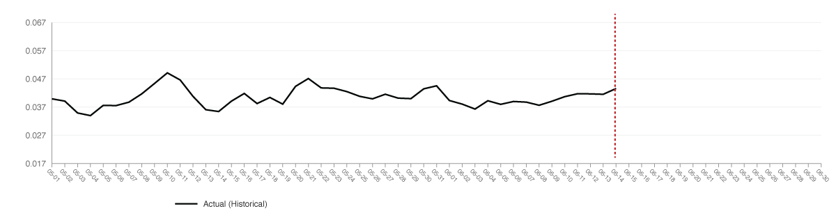
Figure 1: The 1D View of Historical Values
The chart appears one-dimensional. The record is not. Every observation in the record carries two coordinates: the dim 4 Perspective value and the dim 6 Timeline calendar date. The record is bivariate at the data level, a sequence of (value, date) pairs that locates each observed outcome at a specific calendar position. The third dimension, dim 5 Probability, was structurally present at the moment of observation but resolved into the single observed value when the observation occurred. The record carries dim 4 and dim 6 as inputs; dim 5 was collapsed at observation.
The chart and the methods built on it engage only the dim 4 channel. The dim 6 coordinate sits as a label on the horizontal axis rather than as substantive input to the operation.
Neither dimension is lost. The dim 6 calendar date is present in the record at every observation. The dim 5 Probability is recoverable from the record as a Calibrated Probability Band at each seasonal position, built from the empirical distribution of values across past cycles. Recovery requires an operation that engages both dimensions structurally.
Univariate Point Prediction Operations (UU Operations) are the methods built on this one-dimensional reading of the record. The category is exhaustive: ARIMA, exponential smoothing, Holt-Winters, state space models, GARCH and its variants, Prophet, the autoregressive neural architectures from RNN through LSTM and GRU to the transformer-based time series models, the vector autoregressions and other multivariate methods, and the deep learning architectures marketed as probabilistic forecasters are all UU Operations. The distinctions used to differentiate these tools are subordinate to the structural classification. Univariate versus multivariate, parametric versus nonparametric, statistical versus machine learning, point versus probabilistic, classical versus neural: each describes how a method computes its output. None changes the fact that every method operates on a univariate input and produces a point estimate.
Each UU Operation takes the bivariate historical record and converts it into an atemporal sequence. The dim 6 temporal coordinate is discarded and replaced with sequential indexing, integers counting observations in the order they arrived. The output is a univariate sequence of values located at integer positions with no calendar meaning. A univariate operation is then performed on this sequence, generating a single value at the next sequential position. The output is a Prediction.
The dimensional content drops out at two stages. Dim 5 Probability was collapsed at observation, before any UU Operation began. Dim 6 Timeline is discarded at the UU Operation itself, when the temporal coordinate is replaced by sequential indexing. By the time the operation produces an output, two of the three dimensions required for a Forecast are absent from the output. No operation downstream of the discard can restore what the discard removed.
Figure 2 shows the historical record with the Calibrated Probability Bands recovered around each observation, locating each historical dim 4 value within the bands at its dim 6 calendar position. The exceedance is a historical value that broke through both the 85% and 95% bands, landing in the deep tail at that seasonal position. It is the rare event the calibrated rate structurally predicts, not an anomaly against the band. A backtest fit to this record could not exhibit this exceedance: the fitting process would either widen the bands to contain it or adjust parameters until the deviation disappeared, and neither happened here.
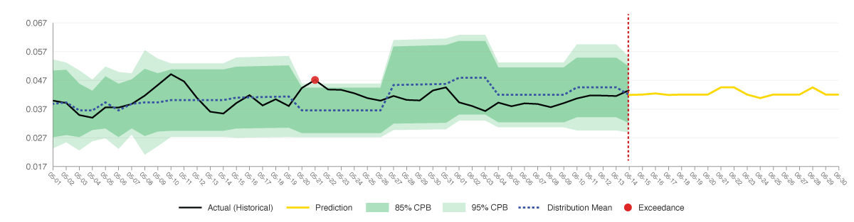
Figure 2: Historical {4,5,6} Recovery Against the Prediction
The bivariate input has been extended to its full {4,5,6} structure. The Prediction extending into the forecast horizon, by contrast, structurally carries no Calibrated Probability Band and no dim 6 engagement. The calendar dates beneath the Prediction line are assigned to the integer sequence positions by the plotting software after the operation completes; they are not structural outputs of the construction. The categorical asymmetry between the historical and forecast sides of the chart is the structural failure that produces every Prediction the field generates.
Temporal Structural Forecasting (TSF) is the construction that resolves the failure. TSF performs two orthogonal UU Operations on two structurally distinct axes: one UU Operation along the dim 4 sequential timeline, a second UU Operation along the dim 6 seasonal timeline. The dim 6 temporal coordinate is preserved at the input stage and used substantively to assign each observation to its seasonal positions across the cycles that organize the underlying process. The two univariate operations are then combined via Orthogonal Projection, producing an output that is no longer restricted to dim 4. The Calibrated Probability Band at each future position is recovered as the empirical distribution of forecast-actual differences across seasons at that position; the dim 6 calendar coordinate is preserved as the structural anchor of the band. The output is a {4,5,6} Forecast object at each future position: a dim 4 value, a Calibrated Probability Band, and a dim 6 calendar coordinate together. Figure 3 shows the full {4,5,6} Forecast across the historical and forecast regions.
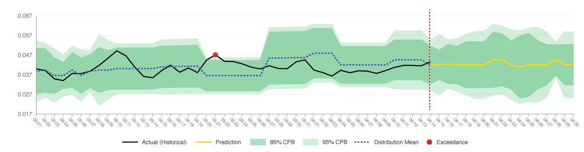
Figure 3: The {4,5,6} Forecast
The Calibrated Probability Bands continue across the boundary; the dim 4 values and the dim 6 calendar coordinates are preserved through the entire record. The Forecast carries the same structural form as the input: a value, a band, and a calendar coordinate at every position. The categorical asymmetry of Figure 2 is resolved.
Exceedance Signals and the Map of Normal
The assumption underlying forecasting is that the operator needs to know the future in order to act. The assumption is partially correct. A Forecast does tell the operator what to expect, by specifying what normal looks like at every future position. But decisions are made in the present, against current conditions, and the operator cannot act in the future. The structural question is therefore not, “When will conditions change?” but, “Is now normal?”
The {4,5,6} Forecast answers the structural question by supplying a reference frame against which any position can be evaluated. The operational name for this reference frame is the Map of Normal. The Map is the CPB structure named for what it does: it specifies what normal looks like at every position across the forecast horizon.
The Map is generated forward in time. Depending on the application, the operator receives a Map covering the week, month, or quarter ahead, with the CPB at every position committed in advance and locked against retroactive adjustment. The Map’s authority comes from its calibration: the bands have delivered the empirical coverage rates they claim across the historical record.
Actuals overlay onto the Map as they arrive. Each actual is immediately classifiable as inside the bands (normal at that position) or outside them (an exceedance). An exceedance is the structural signal that now is not normal. The deviation is meaningful by construction, and the signal is the action trigger.
Planning and acting operate on the Map orthogonally. Planning is forward-looking: it uses the Map’s calibrated structure to prepare the operator’s state for the horizon, with positions sized against band widths, resources staged against measured variability, contracts priced into the calibrated probability content. Acting is present-state: it compares the current actual against the current CPB and asks whether now is normal. Inside the band, no action is indicated. Outside the band, the exceedance triggers action. The two operations run continuously and independently against the same Map; neither requires the other.
The Prediction regime conflates these orthogonal operations and supports neither. The Prediction has no reference frame to plan against and no anchor for evaluating the present. The conventional framing tries to make a single forecasted number serve both operations and delivers neither.
Forecasting vs. Fitting: Why Historical Results Are Not Backtests
Historical Results is a category that has not previously been available. UU Operations produce backtests, the construction of which is described below, and the term “historical results” has been used loosely for what are structurally backtest outputs. The {4,5,6} Forecast produces Historical Results in the literal sense: a record of Forecasts generated under the same constraints that govern live operation, verified against the actuals at each position. The distinction is categorical and holds across every application.
UU Operations perform fitting, not forecasting. A model is tuned against a training segment of historical data until its output matches the observed values. The tuned model is then graded against a held-out segment, and the resulting statistics describe how well the fit generalizes. Forward expectations are projected from the held-out performance, on the assumption that the fit will continue to behave as it did on the data it was tested against.
Forecasting is structurally different. Every Forecast in the Historical Results was generated using only data preceding its position, with no access to data from positions after it. No parameter at any position was informed by data after that position. Nothing was held out because nothing was fit. The Historical Results are a series of Forecasts constructed under live-operation constraints, with the outcomes at each position then compared against the Forecast that had been generated for it.
The Temporal Firewall enforces this structurally. No operation at any historical position has access to data from positions later than itself. A backtest cannot enforce this firewall because backtests require the holistic optimization that violates it. A {4,5,6} Forecast cannot violate it because the construction generates each position from the data preceding it, exactly as live operation does.
The empirical signature is the exceedance pattern. A fit cannot contain visible exceedances against its own bands. If a value lands outside the bands during fitting, the bands widen until the value is contained, or the parameters adjust until the deviation disappears. The exceedance leaves no trace in the record the fit produces because the fit is optimizing against that record. A Forecast has no mechanism to retroactively adjust a band already committed. When an actual lands outside the band, the exceedance stays in the record. Visible exceedances at the rates the bands predict are direct empirical evidence that the construction is forecasting, not fitting.
The operational consequence is asymmetric. A backtest overstates live performance because the optimization that produced it does not transfer to live data. Historical Results match live performance because the historical construction is identical to the live construction. The forward expectation set by Historical Results is structurally honest. The forward expectation set by a backtest is structurally inflated.
The pattern is documented in quantitative finance specifically. The gap between published backtest performance and subsequent live performance is large and well-characterized, and the academic literature on backtest overfitting bias has quantified the inflation across decades of strategy reporting. The same structural reasons predict that {4,5,6} Forecast Historical Results will not exhibit the pattern. The Historical Results presented for any TSF application are not backtests, are not subject to the documented inflation, and represent how the construction actually behaves operationally.
Temporal Structural Forecasting: Dim 6 Seasons and the Calibrated Probability Bands
The Calibrated Probability Band is empirical content. The 85% band at a given position contains 85% of the values the historical record produced at that position; the 95% band contains 95%. The label and the coverage rate match because the band is built from the values themselves, indexed by their dim 6 seasonal position in the record. The dim 6 seasons are the structural prerequisite for the dim 5 CPB.
A season is a defined position within the historical record that recurs across the record, and the values at the same seasonal position across the record form a coherent empirical distribution. The seasonality UU Operations recognize is calendar-based: months, weeks, days of the week. These calendar seasons are visible to the naked eye, and they are the only seasonality UU Operations have been able to engage substantively. The temporal structure that drives most real-world data is not calendar-based. It runs through complex, irregular seasons whose positions recur across the historical record but do not align to the calendar’s regular partitions. These seasons are invisible to the naked eye and undetectable by AI applied to the calendar coordinate alone.
TSF Inc. has invented a Microscope for Time: a library of seasonal lenses that read the historical record through complex, irregular seasonal structures the calendar cannot represent. Each lens is a structurally distinct partition of the record into seasons, and each partition produces a different set of empirical distributions at each seasonal position. What the calendar makes invisible, the lenses make structurally engageable.
The {4,5,6} Forecast is produced by Orthogonal Projection across two axes: the dim 4 sequential axis carrying chronological position, and the dim 6 seasonal axis carrying position within the lens’s seasonal structure. The output at each forward position is a {4,5,6} Forecast object: a dim 4 value, a dim 5 CPB calibrated from the empirical distribution at the corresponding seasonal position across the historical record, and a dim 6 calendar coordinate. The construction has no parameter optimization stage. The empirical distributions are computed directly from the historical record, and every component is structurally locked against retroactive adjustment.
Empirical Results: Exploitable Temporal Structure in Equity Returns
Equity returns are widely treated as the hardest forecasting domain. The Efficient Market Hypothesis treats them as structurally unforecastable; decades of tactical strategies have failed to produce statistically significant timing performance; backtested signals fail when faced with live data, and the field has concluded that the failure is intrinsic to the asset class. The structural argument developed above predicts the opposite: if dim 6 seasonal structure makes the dim 5 CPB possible, and if equity prices carry dim 6 seasonal structure recoverable through the TSF construction, the temporal structure is exploitable and the CPB is the operational mechanism through which exploitation occurs.
The {4,5,6} Forecast generates a CPB at each forward position. The lower band is the structural specification of an abnormally low price at that position; the upper band, an abnormally high price. Equity profit requires buying low and selling high, and the CPB is the structural definition of what low and high mean at each calendar position. The lower band is committed in advance as a Buy Limit Order at the calculated price, placed before the trading window opens. The order fills if the intraday low touches the order price during the window, and expires unfilled if it does not. Each filled position carries a 5% profit target and a forced exit at the maximum hold period. Entry is structural, exit is structural, and nothing about the operation is discretionary.
The construction was applied to 346 S&P 500 constituents across all 11 GICS sectors over the 10-year period from 2016 through 2025, under a preregistered methodology (https://doi.org/10.5281/zenodo.18188491). The full parameter space of the study contains 1,386 permutations: 6 factor strategies × 7 forecast model specifications × 3 confidence thresholds. No permutation was discarded; every result entered the published record.
The single worst-performing permutation in the parameter space achieves a 67.7% win rate (the percentage of filled positions that exited with a positive net return), with a p-value of 3.33 × 10⁻¹⁷. That worst case is more statistically significant than virtually any published finding in the financial economics literature, and it is the worst of 1,386 configurations rather than a selected one. Of the 1,386 permutations, 1,219 (88.0%) achieve win rates at or above 75%; 820 (59.2%) exceed 80%; 1,256 (90.6%) produce p-values below 10-30.
The 2022 bear market provides the adverse-condition evidence. The S&P 500 returned -18.1% for the calendar year. Of 14 TSF factor portfolios tested across the period, 10 posted positive returns. Sub 1 Beta Swing delivered +37.3% and Energy Swing delivered +33.8%, against the benchmark’s -18.1%. Portfolio exposure was higher in 2022 than the full-period average across nearly every configuration; the outperformance was not the result of defensive positioning. Each filled position was entered at the lower CPB band, and the 5% profit target was reached on the majority of those positions even as the broader market declined.
Across the full 10-year study, filled positions reach the 5% profit target 80% of the time. The remaining 20% exit through the forced close at losses averaging -12% to -27% depending on the sector. The losses are larger per position than the wins, but there are far fewer of them, and the portfolio profits on the volume of small wins. The conventional systematic model is the opposite shape: a 30–40% win rate carried by occasional large winners. The TSF construction inverts it.
These are Historical Results, not backtests. Each Forecast in the record was generated using only data preceding its position, under the Temporal Firewall established above; the historical construction is structurally identical to live operation.